1. 伝達関数と時間応答

1-1. インパルス応答から伝達関数

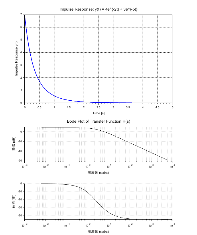
インパルス応答が、$$y(t) = 4e^{-2t} + 3e^{-5t}$$であるとき、システムの伝達関数を求めよ。

解答例：インパルス応答が\(y(t) = 4e^{-2t} + 3e^{-5t}\)なので、このラプラス変換が伝達関数となる。$$G(s) = \mathcal{L}\{g(t)\} = 4\mathcal{L}\{e^{-2t}\} + 3\mathcal{L}\{e^{-5t}\} = \frac{4}{s+2} + \frac{3}{s+5} = \frac{7s + 26}{(s+2)(s+5)}$$

※Scilabスクリプトと実行結果（インパルス応答波形と伝達関数のボード線図を図１）に示す。簡単なスクリプトでインパルス応答波形とボード線図を描けるが、インパルス応答から伝達関数の変換は、基本的に手計算となる。（インパルス応答波形から2次系モデルフィッティングなどで伝達関数を推定する方法はある。）

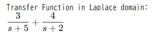
※Pythonでは、ラプラス変換を実行できるので、インパルス応答の式から伝達関数の導出ができる。

1-2. 伝達関数からインパルス応答

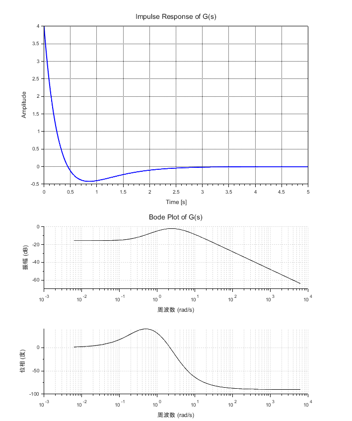
伝達関数が、$$G(s) = \frac{4s+1}{(s+2)(s+3)}$$であるときのインパルス応答を求めよ。

解答例：伝達関数の逆ラプラス変換がインパルス応答である。まず、伝達関数\(G(s)\)を部分分数展開する。$$G(s) = \frac{4s+1}{(s+2)(s+3)} = \frac{a}{s+2} + \frac{b}{s+3}$$ \(a,\;b\)は、展開定理を使って求める。$$a = (s+2)G(s)|_{s=-2} = \left. \frac{4s+1}{s+3}\right|_{s=-2}=-7 \\ b=(s+3)G(s) |_{s=-3} = \left. \frac{4s+1}{s+2} \right|_{s=-3} = 11$$よって、インパルス応答は、$$y(t) = \mathcal{L}^{-1}\{G(s)\}=\mathcal{L}^{-1} \left[-\frac{7}{s+2} + \frac{11}{s+3}\right] \\ =-7\mathcal{L}^{-1}\left[ \frac{1}{s+2}\right] + 11\mathcal{L}^{-1}\left[\frac{1}{s+3}\right] = -7e^{-2t} + 11e^{-3t}$$である。

※Scilabスクリプトとその実行結果（インパルス応答波形と伝達関数のボード線図を図２）に示す。

1-3. 伝達関数からステップ応答

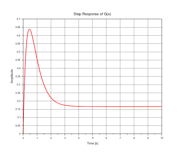
伝達関数が、$$G(s) = \frac{4s+1}{(s+2)(s+3)}$$であるときのステップ応答を求めよ。

解答例：入力\(u(t)\)が単位ステップ信号とすると、そのラプラス変換は、$$U(s) = \mathcal{L}\left[u(t)\right] = \frac{1}{s}$$である。出力は、$$Y(s)=G(s)U(s)=G(s)\frac{1}{s} = \frac{4s+1}{s(s+2)(s+3)}$$である。これを逆ラプラス変換することで、ステップ応答\(y(t)\)が得られる。まず、\(Y(s)\)を部分分数展開する。$$Y(s) = \frac{4s+1}{s(s+2)(s+3)} = \frac{a}{s} + \frac{b}{s+2} + \frac{c}{s+3}$$で \(a,\;b\;c\)は、展開定理を使って求める。$$a = sY(s)|_{s=0} =\left. \frac{4s+1}{(s+2)(s+3)}\right|_{s=0}=\frac{1}{6} \\b= (s+2)Y(s)|_{s=-2} =\left. \frac{4s+1}{s(s+3)}\right|_{s=-2}=\frac{7}{2} \\ c=(s+3)Y(s)|_{s=-3} = \left. \frac{4s+1}{s(s+2)}\right|_{s=-3}=-\frac{11}{3}$$よって、ステップ応答は、$$y(t)= \mathcal{L}^{-1}\left[Y(s)\right] = \frac{1}{6}\mathcal{L}^{-1}\left[\frac{1}{s}\right] +\frac{7}{2}\mathcal{L}^{-1}\left[\frac{1}{s+2}\right] - \frac{11}{3}\mathcal{L}^{-1}\left[\frac{1}{s+3}\right] \\= \frac{1}{6} +\frac{7}{2}e^{-2t} - \frac{11}{3}e^{-3t}$$となる。

※Scilabスクリプトとその実行結果（ステップ応答波形を図３）に示す。

1-4. RC直列回路の伝達関数

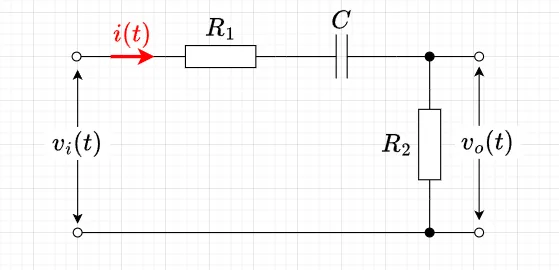
図４に示すRC直列回路において、\(v_i(t)\)[V]を入力信号、\(v_o(t)\)[V]を出力信号としたときの伝達関数を求めよ。ただし、\(t=0\)においてコンデンサ\(C\)の電荷は\(0\)であるとする。

解答例：回路に流れる電流を\(i(t)\)[A]とすると、式(1)が成り立つ。$$R_1 i(t) + \frac{1}{C}\int_0^t i(\tau) d\tau + v_o(t) = v_i(t) \;\;\;\cdots (1)$$また、$$v_o(t) = R_2 i(t) \;\;\; \cdots (2)$$である。式(1),(2)を初期値\(0\)でラプラス変換すると、$$R_1 I(s) + \frac{1}{Cs} I(s) + V_o(s) = V_i(s), \quad V_o(s) = R_2 I(s)$$となる。ここで、\(I(s),\;V_i(s),\;V_o(s)\)は\(i(t),\; v_i(t),\; v_o(t)\)のラプラス変換である。ラプラス変換した式を\(I(s)\)を消去するように整理すると、$$(R_1 C s +1 +R_2 C s)V_o(s) = R_2 C s V_i(s)$$となる。従って、伝達関数は、$$G(s) = \frac{V_o(s)}{V_i(s)} = \frac{R_2 Cs}{(R_1 + R_2)C s +1}$$である。

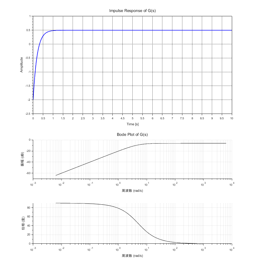
※Scilabスクリプトにより、この伝達関数のボード線図、インパルス応答を求める。ただし、\(R_1 = R_2 = 100\;k\Omega,\;\;\;C=1\;\mu F\)とする。このパラメータの場合、\(G(s)=s/(2s+10)\)となる。図５に実行結果を示す。