7. パルス伝達関数

※離散時間系に関しては、 4. 連続時間システムの離散化 を参照願います。

7-1. 差分方程式からパルス伝達関数へ

離散時間システムの差分方程式が式(1)で与えられている。このシステムのパルス伝達関数を求めよ。$$y(k+n) + a_1y(k+n-1) + \cdots + a_{n-1}y(k+1) +a_n y(k) \\ = b_0 u(k+m) + b_1 u(k+m-1) + \cdots + b_m u(k) \quad(n \gt m) \;\;\; \cdots (1)$$

解答例： 式(1)の両辺を\(\mathcal{Z}\)変換すると、式(2)となる。$$z^n Y(z) + a_1 z^{n-1} Y(z) + \cdots + a_{n-1} z Y(z) + a_n Y(z) \\= b_0 z^m U(z) + b_1 z^{m-1} U(z) + \cdots +b_m U(z) \;\;\; \cdots (2)$$式(2)より、パルス伝達関数\(G(z)\)は、$$G(z) = \frac{Y(z)}{U(z)} = \frac{b_0 z^m + b_1 z^{m-1} + \cdots + b_{m-1} z + b_m}{ z^n + a_1 z^{n-1} + \cdots + a_{n-1} z + a_n} \;\;\; \cdots (3)$$となる。\(z\)は１サンプル進める演算子とみなしてよい。なお、伝達関数を求める場合の\(\mathcal{Z}\)変換では、初期値は\(0\)とする。また、式(3)で分母分子を\(z^n\)で割り、式(4)の形式で表すことも多い。$$G(z) = \frac{b_0 z^{-n+m} + b_1 z^{-n+m-1} + \cdots + b_{m-1}z^{-n+1} + b_m z^{-n}}{ 1 + a_1 z^{-1} + \cdots + a_{n-1} z^{-n+1} + a_n z^{-n}} \;\;\; \cdots (4)$$

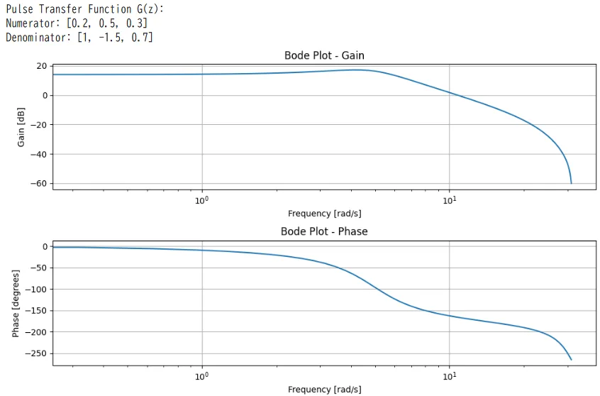
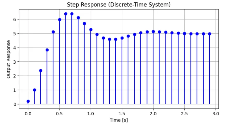
※Pythonによる差分方程式からパルス伝達関数を求めるスクリプトを示す。また、ボード線図、ステップ応答も描画する。

import numpy as np
import matplotlib.pyplot as plt
from scipy.signal import dlti, dstep, dbode
# Parameter settings
# Coefficients (Example: second-order system)
a_coeffs = [1, -1.5, 0.7]  # Coefficients a_n, a_{n-1}, ..., a_1 (LHS)
b_coeffs = [0.2, 0.5, 0.3] # Coefficients b_m, b_{m-1}, ..., b_0 (RHS)
# Sampling period
T = 0.1
# Create discrete-time transfer function
system = dlti(b_coeffs, a_coeffs, dt=T)
# Print pulse transfer function
print("Pulse Transfer Function G(z):")
print(f"Numerator: {b_coeffs}")
print(f"Denominator: {a_coeffs}")
# Bode plot
w, mag, phase = dbode(system)
plt.figure(figsize=(10, 6))
plt.subplot(2, 1, 1)
plt.semilogx(w, mag)
plt.xlabel('Frequency [rad/s]')
plt.ylabel('Gain [dB]')
plt.title('Bode Plot - Gain')
plt.grid()
plt.subplot(2, 1, 2)
plt.semilogx(w, phase)
plt.xlabel('Frequency [rad/s]')
plt.ylabel('Phase [degrees]')
plt.title('Bode Plot - Phase')
plt.grid()
plt.tight_layout()
plt.show()
# Step response
t, y_step = dstep(system,n=30)
plt.figure(figsize=(8, 4))
markerline, stemlines, baseline = plt.stem(t, np.squeeze(y_step), basefmt=" ")
plt.setp(markerline, color='b', marker='o')  # Set point color and marker
plt.setp(stemlines, color='b', linestyle='-')  # Set stem color and line style
plt.xlabel('Time [s]')
plt.ylabel('Output Response')
plt.title('Step Response (Discrete-Time System)')
plt.grid()
plt.show()

7-2. パルス伝達関数から差分方程式へ

離散時間システムのパルス伝達関数が式(5)で与えられている。このシステムの差分方程式を求めよ。$$G(z) = \frac{b_1 z^{n-1} + b_2 z^{n-2} + \cdots + b_{n-1}z + b_n}{z^n + a_1 z^{n-1} + \cdots + a_{n-2} z^2 + a_{n-1} z+ a_n} \;\;\; \cdots (5)$$

解答例：　式(5)の分母分子に\(z^{-n}\)を掛けると$$G(z) = \frac{b_1 z^{-1} + b_2 z^{-2} + \cdots + b_{n-1}z^{-n+1} + b_n z^{-n}}{1 + a_1 z^{-1} + \cdots + a_{n-2} z^{-n+2} + a_{n-1} z^{-n+1}+ a_n z^{-n}}$$となる。\(G(z) = Y(z)/U(z)\)なので、$$Y(z)\left\{1 + a_1 z^{-1} + \cdots + a_{n-2} z^{-n+2} + a_{n-1} z^{-n+1}+ a_n z^{-n}\right\} \\= U(z)\left\{b_1 z^{-1} + b_2 z^{-2} + \cdots + b_{n-1}z^{-n+1} + b_n z^{-n}\right\} \\ Y(z) + a_1 z^{-1}Y(z) + \cdots + a_{n-2} z^{-n+2}Y(z) + a_{n-1} z^{-n+1}Y(z)+ a_n z^{-n}Y(z) \\= b_1 z^{-1}U(z) + b_2 z^{-2}U(z) + \cdots + b_{n-1}z^{-n+1}U(z) + b_n z^{-n}U(z)$$ \(z^{-1}\)を１サンプル遅らせる演算子と考えて逆\(\mathcal{Z}\)変換すると、$$y(k) + a_1y(k-1) + \cdots +a_{n-2} y(k-n+2) +a_{n-1}y(k-n+1) + a_n y(k-n) \\ = b_1 u(k-1) + b_2 u(k-2) + \cdots + b_{n-1}u(k-n+1) + b_n u(k-n)$$よって、$$y(k) = -a_1y(k-1) - \cdots -a_{n-2} y(k-n+2) -a_{n-1}y(k-n+1) - a_n y(k-n) \\+ b_1 u(k-1) + b_2 u(k-2) + \cdots + b_{n-1}u(k-n+1) + b_n u(k-n) $$となる。

※Pythonのスクリプトと結果を示す。

import numpy as np
from scipy.signal import dlti
def transfer_function_to_difference_eq(b_coeffs, a_coeffs):
    """Convert pulse transfer function to difference equation."""
    # Normalize coefficients (make a[0] = 1 if needed)
    a_coeffs = np.array(a_coeffs)
    b_coeffs = np.array(b_coeffs)
    if a_coeffs[0] != 1:
        b_coeffs = b_coeffs / a_coeffs[0]
        a_coeffs = a_coeffs / a_coeffs[0]
    n = len(a_coeffs) - 1
    m = len(b_coeffs) - 1
    # Print the difference equation
    print("\nDifference Equation:")
    eq_str = ""
    # Output terms
    for i in range(1, n + 1):
        eq_str += f"- {a_coeffs[i]:.3f} y[k-{i}] " if a_coeffs[i] != 0 else ""
    # Input terms
    for i in range(m + 1):
        eq_str += f"+ {b_coeffs[i]:.3f} u[k-{i}] " if b_coeffs[i] != 0 else ""
    # Final equation
    eq_str = f"y[k] = {eq_str.strip()}"
    print(eq_str)
# Example coefficients
b_coeffs = [0.2, 0.5, 0.3]  # Numerator coefficients (b1, b2, ..., bn)
a_coeffs = [1, -1.5, 0.7]   # Denominator coefficients (1, a1, ..., an)
# Convert transfer function to difference equation
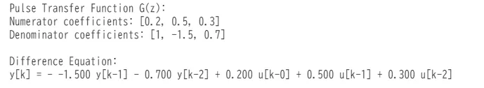
print("Pulse Transfer Function G(z):")
print(f"Numerator coefficients: {b_coeffs}")
print(f"Denominator coefficients: {a_coeffs}")
transfer_function_to_difference_eq(b_coeffs, a_coeffs)

7-3. 連続時間系の伝達関数からパルス伝達関数

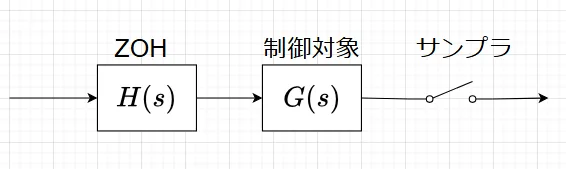
解答例： ZOHの伝達関数\(H(s)\)は、$$H(s) = \frac{1-e^{-Ts}}{s} = \left(1-z^{-1}\right)\frac{1}{s}$$である。従って、ZOHの入力からサンプラの出力までのパルス伝達関数\(G(z\)は、$$G(z) = \left(1-z^{-1}\right)\mathcal{Z}\left[\frac{G(s)}{s}\right] $$である。$$\mathcal{Z}\left[\frac{G(s)}{s}\right] = \mathcal{Z}\left[\frac{1}{s(as+1)}\right] \\= \mathcal{Z}\left[\frac{1}{s} - \frac{1}{s+\frac{1}{a}}\right] = \frac{z}{z-1} - \frac{z}{z-e^{-\frac{T}{a}}}$$よって、$$G(z) = (1-z^{-1})\left[\frac{z}{z-1} - \frac{z}{z-e^{-\frac{T}{a}}}\right] = 1- \frac{z-1}{z-e^{-\frac{T}{a}}} =\frac{1-e^{-\frac{T}{a}}}{z-e^{-\frac{T}{a}}}$$となる。

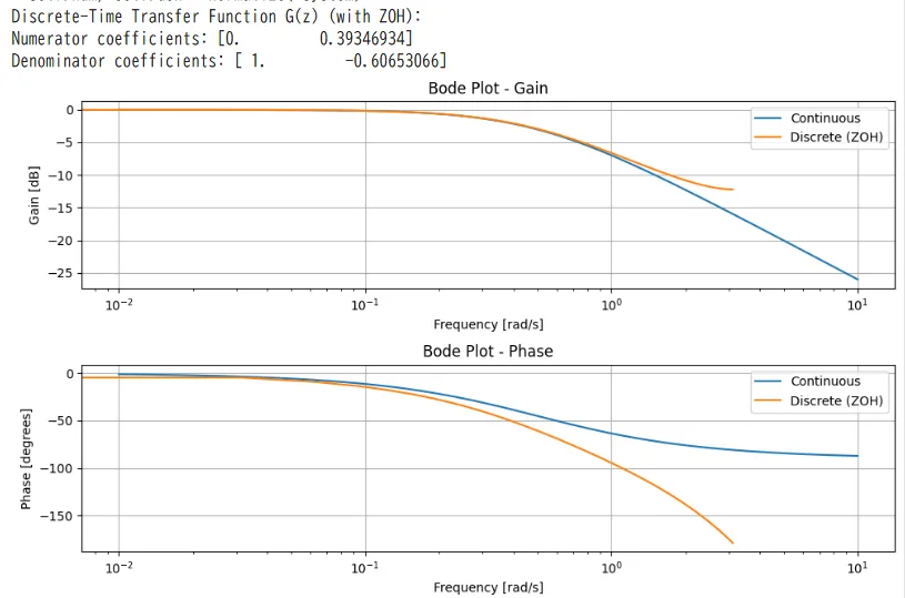
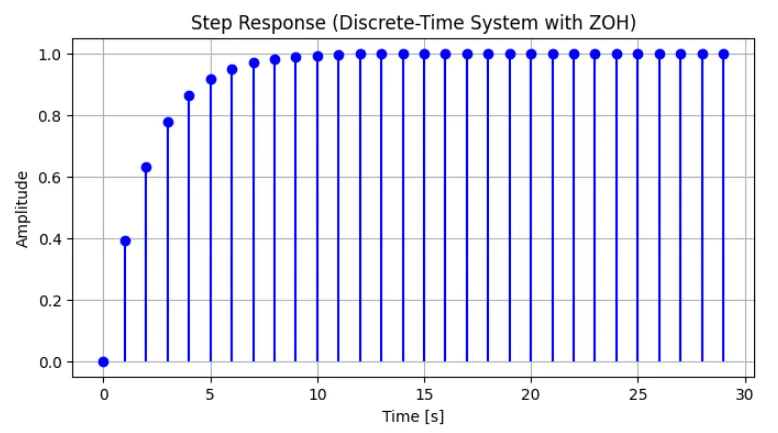
※連続時間系伝達関数\(G(s)\)をZOHを付けた離散時間系伝達関数\(G(z)\)に変換し、ボード線図、ステップ応答を求めるPythonスクリプトとその実行結果を示す。

import numpy as np
import matplotlib.pyplot as plt
from scipy.signal import cont2discrete, dlti, dstep, dbode, lti #import dbode
# Parameters
a = 2                      # System parameter
T = 1.0                   # Sampling period
# Continuous-time transfer function G(s)
num = [1]                  # Numerator
den = [a, 1]               # Denominator
# Discretize with ZOH G(z)
system_cont = (num, den)
system_discrete = cont2discrete(system_cont, T, method='zoh')
# Extract numerator and denominator coefficients for G(z)
num_z, den_z = system_discrete[0].flatten(), system_discrete[1].flatten()
# Create discrete system
Gz = dlti(num_z, den_z, dt=T)
# Print the discrete transfer function
print("Discrete-Time Transfer Function G(z) (with ZOH):")
print(f"Numerator coefficients: {num_z}")
print(f"Denominator coefficients: {den_z}")
# Bode plot (Continuous and Discrete)
w_cont, mag_cont, phase_cont = bode(lti(num, den))
# Use dbode for the discrete-time system
w_disc, mag_disc, phase_disc = dbode(Gz) # Changed bode to dbode
plt.figure(figsize=(10, 6))
plt.subplot(2, 1, 1)
plt.semilogx(w_cont, mag_cont, label='Continuous')
plt.semilogx(w_disc, mag_disc, label='Discrete (ZOH)')
plt.xlabel('Frequency [rad/s]')
plt.ylabel('Gain [dB]')
plt.title('Bode Plot - Gain')
plt.grid()
plt.legend()
plt.subplot(2, 1, 2)
plt.semilogx(w_cont, phase_cont, label='Continuous')
plt.semilogx(w_disc, phase_disc, label='Discrete (ZOH)')
plt.xlabel('Frequency [rad/s]')
plt.ylabel('Phase [degrees]')
plt.title('Bode Plot - Phase')
plt.grid()
plt.legend()
plt.tight_layout()
plt.show()
# Step response
t_disc, y_disc = dstep(Gz,n=30)
plt.figure(figsize=(8, 4))
markerline, stemlines, baseline = plt.stem(t_disc, np.squeeze(y_disc), basefmt=" ")
plt.setp(markerline, color='b', marker='o')
plt.setp(stemlines, color='b', linestyle='-')
plt.xlabel('Time [s]')
plt.ylabel('Amplitude')
plt.title('Step Response (Discrete-Time System with ZOH)')
plt.grid()
plt.show()