8. 離散時間システムの応答

※離散時間システムの応答に関しては、5. 離散時間システムの応答、9. 離散時間システムの構造を参照願います。

8-1. 固有値が正または零の実数

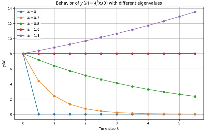
固有値\(\lambda_i\)が正または零の実数のとき、\(\lambda_i^k x_i(0)\)の振る舞いを図示せよ。ただし、\(x_i(0) = 8\)とする。

解答例： 固有値\(\lambda_i\)が正の実数なので、固有値の大きさが１よりも大きい場合は、\(\lambda_i^k\)は発散する。１ならば大きさ１のままである。また、\(0 \lt \lambda_i \lt 1\)ならば零に収束する。また、\(\lambda_i = 0\)ならば、初期値\(x_i(0)\)の値に関係なく、１ステップで\(\lambda_i^k x_i(0)\)は零に収束する。

※Pythonによるスクリプトと実行結果（図１）を示す。

import numpy as np
import matplotlib.pyplot as plt
# Parameters
k = np.arange(0, 6, 0.5)       # Time steps
x0 = 8                         # x_i(0) = 8
# Different eigenvalues
lambdas = [0, 0.3, 0.8, 1.0, 1.1]      # λ_i values to test
# Plotting the behavior
plt.figure(figsize=(10, 6))
for lam in lambdas:
    y_i = x0 * (lam ** k)     # Compute y_i(k) = λ_i^k * x_i(0)
    plt.plot(k, y_i, marker='o', label=f"$\lambda_i = {lam}$")
# Plot settings
plt.xlabel('Time step $k$')
plt.ylabel('$y_i(k)$')
plt.title('Behavior of $y_i(k) = \lambda_i^k x_i(0)$ with different eigenvalues')
plt.axhline(0, color='gray', lw=0.5)
plt.legend()
plt.grid()
plt.show()

8-2. 固有値が複素数

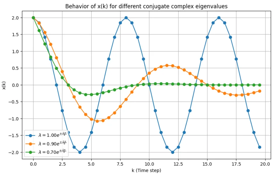
固有値\(\lambda_1,\;\lambda_2\)が共役複素数のとき$$x(k) = \lambda_1^k + \lambda_2^k$$の振る舞いを図示せよ。

解答例： 共役複素数の固有値を極座標形式で表すと$$\lambda_1 = r e^{j \theta},\quad \lambda_2 = r e^{-j \theta}$$ここで、\(r \gt 0,\quad \theta \gt 0\)である。\(x(k)\)の第\(i\)番目の要素は、$$x_i(k) = r^k e^{j(\theta k + \phi_i)} + r^k e^{-j(\theta k + \phi_i)} = 2r^k \cos (\theta k + \phi_i)$$ と表せる。この式から\(0 \lt r \lt 1\)ならば、\(\lim_{k \to \infty} x(k)=0 \) となることがわかる。\(r=1\)ならば持続振動、\(r \gt 1\)ならば発散する。また、\(\theta\)で振動の周期が決まる。

※Pythonによるスクリプトと実行結果（図２）を示す。

import numpy as np
import matplotlib.pyplot as plt
from fractions import Fraction
# Define four sets of conjugate complex eigenvalues
eigenvalues = [
    (1.0 * np.exp(1j * np.pi / 4), 1.0 * np.exp(-1j * np.pi / 4)),
    (0.9 * np.exp(1j * np.pi / 6), 0.9 * np.exp(-1j * np.pi / 6)),
    (0.7 * np.exp(1j * np.pi / 6), 0.7 * np.exp(-1j * np.pi / 6))
]
# Time steps
k = np.arange(0, 20, 0.5)
# Helper function to express angle as a fraction of π
def angle_to_pi_fraction(theta):
    frac = Fraction(theta / np.pi).limit_denominator(100)
    if frac.denominator == 1:
        return f"{frac.numerator}\pi"
    else:
        return f"\\frac{{{frac.numerator}\pi}}{{{frac.denominator}}}"
# Plot the results
plt.figure(figsize=(10, 6))
for idx, (lambda1, lambda2) in enumerate(eigenvalues):
    x_k = lambda1**k + lambda2**k  # Compute sequence
    r = np.abs(lambda1)
    theta = np.angle(lambda1)
    # Show eigenvalues in exponential form with π as a fraction
    plt.plot(k, x_k.real, marker='o',
             label=f"$\lambda = {r:.2f} e^{{\pm i
{angle_to_pi_fraction(theta)}}}$")
# Labels and legend
plt.xlabel("k (Time step)")
plt.ylabel("x(k)")
plt.title("Behavior of x(k) for different conjugate complex eigenvalues")
plt.legend()
plt.grid()
plt.show()

8-3. 状態空間表現における離散化と時間応答

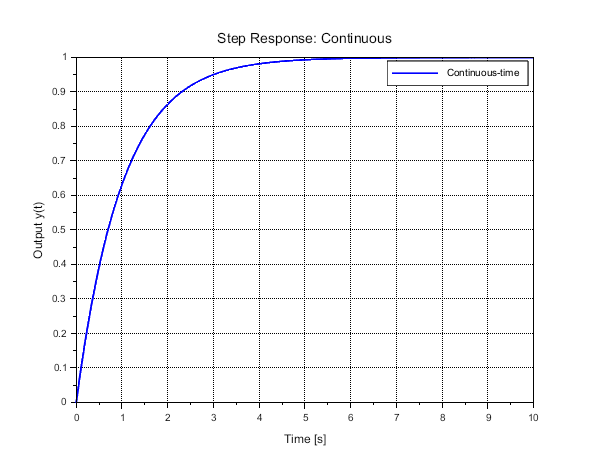
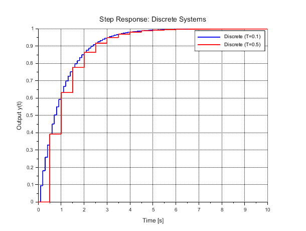
連続時間システム$$\dot x(t) = \begin{bmatrix} 0 & 1 \\ 0 & -1 \end{bmatrix}x(t) + \begin{bmatrix} 0 \\ 1 \end{bmatrix} u(t)$$をサンプリング周期\(T=0.1, \; 0.5\) で離散化し、ステップ応答を求めよ。

解答例： 連続時間システムが状態方程式、$$\dot x(t)=A x(t) + b u(t)$$で表されるとすると、その離散時間システムは、$$x(k+1) = Fx(k) + gu(k) , \quad F = e^{AT}, \quad g = \int_0^T e^{A \tau} d \tau b$$で与えられる。\(e^{At}\)は、$$e^{At} = \mathcal{L}^{-1}\left[(sI -A)^{-1}\right]$$なので、$$A = \begin{bmatrix} 0 & 1 \\ 0 & -1 \end{bmatrix}$$より、$$(sI-A)^{-1} = \begin{bmatrix} s & -1 \\ 0 & s+1 \end{bmatrix}^{-1} = \frac{1}{s(s+1)}\begin{bmatrix} s+1 & 1 \\ 0 & s \end{bmatrix} = \begin{bmatrix} \frac{1}{s} & \frac{1}{s(s+1)} \\ 0 & \frac{1}{s+1} \end{bmatrix}$$これを逆ラプラス変換すると、$$e^{At} = \mathcal{L}^{-1}\left[(sI -A)^{-1}\right]=\begin{bmatrix} 1 & 1-e^{-t} \\ 0 & e^{-t} \end{bmatrix}$$よって、$$F=e^{AT} = \begin{bmatrix} 1 & 1-e^{-T} \\ 0 & e^{-T} \end{bmatrix}$$である。また、$$g = \int_0^T e^{A\tau} d\tau b =\int_0^T \begin{bmatrix} 1 & 1-e^{-\tau} \\ 0 & e^{-\tau}\end{bmatrix} d\tau \begin{bmatrix} 0 \\ 1 \end{bmatrix} \\= \begin{bmatrix} T & T-1+e^{-T} \\ 0 & 1-e^{-T}\end{bmatrix}\begin{bmatrix} 0 \\ 1 \end{bmatrix} = \begin{bmatrix} T-1+e^{-T} \\ 1-e^{-T} \end{bmatrix}$$である。

※連続時間システムの離散化と連続時間系と離散時間系のステップ応答を比較するScilabスクリプトとその実行結果（図３,４）を示す。なお、\(T=0.1,\; T=0.5\)にしたときの、\(F,\;g\)の値は、sys_d1, sys_d2 の A(matrix), B(matrix)で与えられる。

// Scilab script to discretize a system and compare step responses
// Clear the environment
clear; clc; clf();
// Define continuous-time system matrices
A = [0, 1; 0, -1];
B = [0; 1];
C = [0, 1];
D = [0];
// Create the continuous-time system
sys_c = syslin('c', A, B, C, D);
// Simulation parameters
t_max = 10;
dt = 0.01;  // Time step for continuous simulation
t_cont = 0:dt:t_max;   // Fine grid for continuous time
// Generate step input
u_cont = ones(size(t_cont, '*'));
// Simulate continuous-time step response using ode
y_cont = csim('step',t_cont,sys_c)
// Discretize the system with different sampling periods
T1 = 0.1;
T2 = 0.5;
sys_d1 = dscr(sys_c, T1);   // Discretize with T=0.1
sys_d2 = dscr(sys_c, T2);   // Discretize with T=0.5
// Time vectors for discrete responses
t_disc1 = 0:T1:t_max;
t_disc2 = 0:T2:t_max;
// Generate discrete step input
u_disc1 = ones(1,size(t_disc1, '*'));
u_disc2 = ones(1,size(t_disc2, '*'));
// Simulate discrete-time step responses using flts
y_disc1 = flts(u_disc1, sys_d1);
y_disc2 = flts(u_disc2, sys_d2);
// Plot results
scf(0);
plot(t_cont, y_cont, 'b-', 'LineWidth', 2);
xlabel('Time [s]');
ylabel('Output y(t)');
title('Step Response: Continuous');
legend('Continuous-time');
xgrid();
scf(1);
plot2d2(t_disc1, y_disc1, style=2, leg='Discrete (T=0.1)');
plot2d2(t_disc2, y_disc2, style=5, leg='Discrete (T=0.5)');
xlabel('Time [s]');
ylabel('Output y(t)');
title('Step Response: Discrete Systems');
legend('Discrete (T=0.1)', 'Discrete (T=0.5)');
xgrid();